Advanced Users’ Guide

ExPRES (Exoplanetary and Planetary Radio Emission Simulator) is a versatile tool that is fully configurable through the simulation run input file. We present here the details of each configuration parameter.

Main Concepts

The ExPRES tool is modeling planetary radio emission observability. It is described in details in [LHC+19]. It is implementing the Cyclotron Maser Instability (CMI) radio emission mechanism [Wu85], which predicts a strongly anisotropic radio source beaming pattern. The beaming pattern is a hollow cone, whose axis is aligned with the local magnetic field direction, and the cone opening angle is related to the unstable particle distribution function properties. ExPRES computes the radio source to observer spatial vector and compares is direction to the modelled radio source beaming pattern.

The ExPRES code configuration requires the definition of:

The celestial bodies involved in the simulation. At least one central body must be defined, which serves as the spatial origin for the simulation. When several bodies are defined, their relative location with the central body must be available either as precomputed data, or through orbital parameters provided in the configuration file.
The location of the observer with respect to the central body. The location data must be available (either as precomputed data, or through parameters provided in the configuration file.
The magnetic field and plasma density models associated to the celestial bodies. Several type of models can be configured. ExPRES is using a set of pre-computed magnetic field lines from a series of magnetic field models. The plasma density models are set through configuration parameters.
The spatial distribution of the radio sources. This location is related to the magnetic field line carrying the unstable particles. The range of radio source frequencies must also be set.
The radio source properties. The radio emission mechanism is defined by a set of parameters characterising the radio source beaming pattern.

The central body is the simulation run spatial origin and its radius sets the units of spatial parameters. The times are given in a UTC scale in the observer’s frame. The time origin of the simulation run is provided in the observer’s definition.

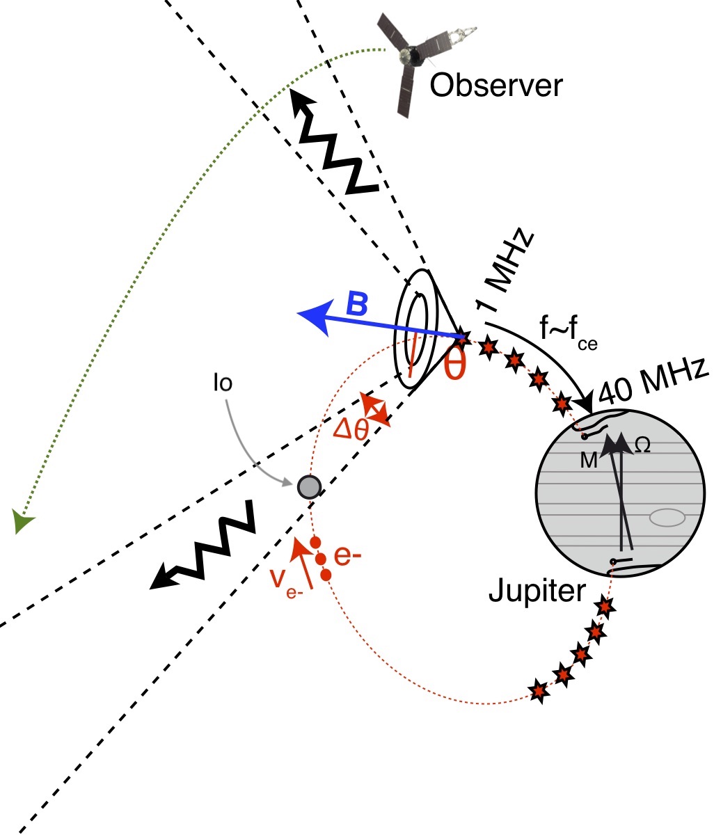
Outline of ExPRES code — **Fig. 1:** Schematic outline of the ExPRES code. The central body here is set up Jupiter and Juno is the observer. The radio sources are placed along the magnetic field line connected to Io. The radio emission beaming pattern model (hollow cone opening angle and thickness) is computed from the magnetic and plasma models. The radio emission observable when the observer is located within the radio source beaming pattern. (Figure adapted from C. Louis, PhD Dissertation, 2018)

All spatial parameters of the simulation configuration (distances, radii, lengths…) must be defined in the same units as that of provided central body radius. Hence, setting the central body radius to 1 implies that all other spatial parameters are provided in units of the central body planetary radii. On the contrary, providing the radius of the central body in km implies that all other spatial parameters must be also provided in km. The recommended convention is to provide all spatial parameters in units of the central body radius. This convention is followed in the examples provided below.

The file output file names are built by ExPRES, using a set up configuration parameters. The general scheme is: expres_{OBS}_{BODY}_{SRC}_{MAG}_{SRC_PROP}_{DATE}_v{VERS}.json. The parts of the template are explained in the table below, with an example using the file: expres_juno_jupiter_io_jrm09_lossc-wid1deg_3kev_20180913_v01.json

Template part	Description	Example
`{OBS}`	Observer name	`juno`
`{BODY}`	Central body name	`jupiter`
`{SRC}`	Radio source driver	`io`
`{MAG}`	Magnetic field model name	`jrm09`
`{SRC_PROP}`	Radio source properties	`lossc-wid1deg_3kev`
`{DATE}`	Simulation date	`20180913`
`{VERS}`	Version of ExPRES	`01`

Simulation Setup

The simulation setup is configured via an ExPRES configuration file (in JSON format), following the ExPRES JSON-Schema v1.3.

Configuration File Description

The ExPRES configuration file should start with the reference to the validation schema to be used. The configuration sections and structure are summarised below:

{
  "$schema": "https://voparis-ns.obspm.fr/maser/expres/v1.2/schema#",
  "SIMU": {...},
  "NUMBER": {...},
  "TIME": {...},
  "FREQUENCY": {...},
  "OBSERVER": {...},
  "SPDYN": {...},
  "MOVIE2D": {...},
  "MOVIE3D": {...},
  "BODY": [{...}, {...}]
  "SOURCE": [{...}, {...}]
}

Each JSON entry shown here is described in the next sections. The BODY section is specific: it is a list of BODY elements, each of which containing a list of DENS elements.

Section	Mandatory in v1.2	Description
SIMU	no	Simulation run description
NUMBER	yes	Number of elements for lists
TIME	yes	Time axis configuration
FREQUENCY	yes	Spectral axis configuration
OBSERVER	yes	Observer’s configuration
SPDYN	yes	Dynamic Spectra output configuration
MOVIE2D	yes	2D movie output configuration
MOVIE3D	yes	3D movie output configuration
BODY	yes	Celestial bodies configuration
SOURCE	yes	Radio Sources configuration

General Parameters

The general parameters cover the time and frequency domain covered by the simulation, allow to give it a name to set the number of objects that will be included in the model. It is composed of 4 sections: SIMU, NUMBER, TIME, FREQUENCY.

Simulation Run Description

The SIMU section contains the simulation run description. It is composed of 2 keywords:

NAME: The name of the simulation
OUT: Output directory location (full path). If this path is empty, the current execution location is used. If this path points a file, the parent directory is selected.

Example: The simulation name is set to Io2015-04-30, and the output directory is defined from the path of the ExPRES configuration file.

"SIMU": {
  "NAME": "Io2015-04-30",
  "OUT": "/Groups/SERPE/SERPE_6.1/Corentin/save/Earth/VIPAL/2015/3kev/Io/Io2015-04-30.json"
},

Simulation List Sizes

The NUMBER section defines maximum numbers of BODY, DENSITY and SOURCE objects, which can be configured in the simulation run. It is composed of 3 keywords:

BODY: The number of planetary bodies in the simulation (e.g., 2 for Jupiter and Io)
DENSITY: The number of plasma density model in the simulation (usually 1 per body)
SOURCE: The number of radio source types in the simulation (usually 1 per interaction and per hemisphere)

Example: We want to define two bodies (Jupiter and Io), two density models (one for Jupiter’s ionosphere, and the other for the Io Torus) and two sets of radio sources (one for each hemisphere).

"NUMBER": {
  "BODY": 2,
  "DENSITY": 2,
  "SOURCE": 2
},

Temporal Axis

The TIME section contains the simulation time configuration. Times are given in minute from the simulation time origin. The time origin is either set by the input ephemeris data or by the input orbital parameters. It is composed of 3 keywords:

MIN: The start time of the simulation (in minutes), usually set to 0.
MAX: The end time of the simulation (in minutes).
NBR: The number of time steps of the simulation.

Example: The simulation starts at the simulation time origin, with 1440 minutes duration (one day), with one step per minute.

"TIME": {
  "MIN": 0,
  "MAX": 1439,
  "NBR": 1440
}

Spectral Axis

The FREQUENCY section contains the simulation spectral configuration. Frequency values are always in MHz units.

The spectral axis can be defined in several ways. The more generic way is to set the spectral axis bounds, the number of steps and the linear and logarithmic scale (see example below). It is also possible to use a predefined set of frequencies, corresponding to an existing instrument. Finally an external file containing a list of frequencies can be provided.

This section is composed of 5 keywords:

TYPE: The spectral axis type. The allowed values are Linear, Log and Pre-Defined.
MIN: The spectral axis lower bound in MHz. Not used when TYPE="Pre-Defined"
MAX: The spectral axis upper bound in MHz. Not used when TYPE="Pre-Defined"
NBR: The number of steps of the spectral axis. Not used when TYPE="Pre-Defined"
SC: In case TYPE="Pre-Defined", the name of the specific spacecraft (not implemented, allowed values TBD), or a list of frequency values.

Example: The simulation spectral axis is a linear scale, ranging from 10 kHz to 44 MHz, with 781 steps.

"FREQUENCY": {
  "TYPE": "Linear",
  "MIN": 0.01,
  "MAX": 44.0,
  "NBR": 781,
  "SC": ""
},

Example: The simulation spectral axis is set of predefined frequencies.

"FREQUENCY": {
  "TYPE": "Pre-Defined",
  "MIN": 0,
  "MAX": 0,
  "NBR": 0,
  "SC": [0.1, 0.2, 0.3, 0.4, 0.5, 0.6, 0.7, 0.8, 0.9, 1, 1.1, 1.2, 1.3, 1.4, 1.5, 1.6, 1.7, 1.8, 1.9, 2,
    2.1, 2.2, 2.3, 2.4, 2.5, 2.6, 2.7, 2.8, 2.9, 3, 3.1, 3.2, 3.3, 3.4, 3.5, 3.6, 3.7, 3.8, 3.9, 4, 4.1,
    4.2, 4.3, 4.4, 4.5, 4.6, 4.7, 4.8, 4.9, 5, 6, 7, 8, 9, 10, 11, 12]
},

Observer Definition

The OBSERVER section contains the observer’s configuration. There are three types of observers, configured by the TYPE keyword:

Fixed observers, whose position does not vary in the reference frame of the simulation;
Orbiter, which moves in the reference frame of the simulation, orbiting around a celestial body;
Pre-Defined observers, which concerns known space mission around celestial bodies.

The observer’s location is provided with respect to the simulation central body, defined in the BODY section.

This section is composed of a series of keywords. The table below provides which keyword shall be used, or left empty, or with a specific value. The following subsections give details for each observer’s type.

Keyword	Observer’s type
`TYPE`	`Fixed`	`Orbiter`	`Pre-Defined`
`EPHEM`	empty	empty	file name or empty
`FIXE_DIST`	distance	`auto`	`auto`
`FIXE_SUBL`	longitude	`auto`	`auto`
`FIXE_DECL`	latitude	`auto`	`auto`
`PARENT`	Reference body name
`SC`	Observer’s name
`SCTIME`	Start time
`SEMI_MAJ`	0	Semi major axis	0
`SEMI_MIN`	0	Semi minor axis	0
`SUBL`	0	Apoapsis longitude	0
`DECL`	0	Apoapsis latitude	0
`PHASE`	0	Phase from apoapis	0
`INCL`	0	Inclination	0

The observer’s name (SC keyword) must be set, and can’t be empty. When TYPE="Pre-Defined" and EPHEM="", the current allowed list of values is: Juno, Earth, Galileo, JUICE, Cassini, Voyager1, Voyager2.

The PARENT keyword must be set to one of the celestial body names defined in the BODY section. Except for specific cases, it is usually the central body name.

The simulation start time (SCTIME keyword) is provided in SCET (spacecraft event time), with a YYYYMMDDHHMMSS format.

Fixed Observer

A fixed observer is configured by a location at the start of the simulation: its distance (FIXE_DIST keyword) to the central body, its sub-longitude in degrees (FIXE_SUBL keyword) and its declination in degrees (FIXE_DECL keyword) in the reference body frame. The location of such an the observer is fixed in an absolute frame centered on the central body. Hence it is not fixed in the central body frame, which is rotating with its sidereal period.

Orbiter

The observer’s orbital parameters are its semi-major (SEMI_MAJ keyword) and semi-minor (SEMI_MIN keyword) axis lengths, its apoapsis sub-longitude (SUBL keyword) and declination (DECL keyword), as well as the inclination of the orbit plane around the semi-major axis (INCL keyword). All angles are provided in the central body reference frame, and at the simulation time origin. Finally, the orbiter position requires the definition of its initial phase (PHASE keyword) on the orbit, i.e., 0 degree is at the apoapsis position.

Pre-Defined

In the case of predefined observers, the code is expecting to have access to ephemeris information. For a set of space missions (Cassini, Voyager1, Voyager2, Juno) or planetary bodies (Earth), the code will call the Miriade ephemph webservice at IMCCE. For all other cases, an ephemeris file extracted from WebGeoCalc shall be provided using the EPHEM keyword.

Example: We configure a simulation with an observer at Earth, with a simulation starting on 2015-04-30T00:00:00.

"OBSERVER": {
  "TYPE": "Pre-defined",
  "EPHEM": "",
  "FIXE_DIST": "auto",
  "FIXE_SUBL": "auto",
  "FIXE_DECL": "auto",
  "PARENT": "Jupiter",
  "SC": "Earth",
  "SCTIME": "201504300000",
  "SEMI_MAJ": 0,
  "SEMI_MIN": 0,
  "SUBL": 0,
  "DECL": 0,
  "PHASE": 0,
  "INCL": 0
},

Example: We configure a simulation from the JUICE spacecraft, providing a WebGeocalc output CSV file.

"OBSERVER": {
  "TYPE": "Pre-Defined",
  "EPHEM": "WGC_StateVector_JUICE_SC_20320111T175800_20320111T185900.csv",
  "FIXE_DIST": "auto",
  "FIXE_SUBL": "auto",
  "FIXE_DECL": "auto",
  "PARENT": "Jupiter",
  "SC": "JUICE",
  "SCTIME": "",
  "SEMI_MAJ": 0,
  "SEMI_MIN": 0,
  "SUBL": 0,
  "DECL": 0,
  "PHASE": 0,
  "INCL": 0
},

Celestial Bodies Definition

The BODY section contains the celestial bodies configuration.

Two types of celestial bodies can be included in the simulations:

Fixed bodies (at least is one needed): the simulation run reference body (MOTION=false);
Orbiting bodies, which can orbit both fixed and orbiting bodies (MOTION=true).

Each body must be given a unique name within the configuration file, since the name is used internally by ExPRES to refer to them. Each body radius must be specified. All distances and scales units must be consistent throughout a configuration file.

Celestial body definitions include the following keywords:

ON: Flag to activate the current body (true or false)
NAME: The name of the current body (must be unique in the configuration file)
RADIUS: The radius of the current body (in consistent units throughout the configuration file)
PERIOD: The sidereal rotation period of the current body (in minutes)
FLAT: The polar flatening ratio of the current body.
ORB_PER: The orbital period according to 3rd Kepler’s law at 1 radius (in minutes)

Example: For Io, we have \(M_{Io} = 8.931 \times 10^{22}~\textrm{kg}\), \(a = 1821 \times 10^{3}~\textrm{m}\) and \(G = 6.674 \times 10^{-11}~\textrm{N}.\textrm{m}^{2}.\textrm{kg}^{-2}\), therefore \(T = \sqrt{\frac{a^{3} * 4 * \pi^{2}}{G * M_{\textrm{Io}}}}*\frac{1}{60} = 105.4~\textrm{min}\)

INIT_AX: The reference longitude (in degrees)
MAG: The internal body magnetic field model (see the Magnetic Field Model section below)
MOTION: Flag to indicate if the current body is moving in the simulation frame (must be false for the central body)
PARENT: Named body, around which the current body is orbiting (must be one of the defined bodies, and must be empty for the central body)
SEMI_MAJ: The semi-major axis orbital parameter of the current body (must be 0 for the central body)
SEMI_MIN: The semi-minor axis orbital parameter of the current body (must be 0 for the central body)
DECLINATION: The declination orbital parameter of the current body (must be 0 for the central body)
APO_LONG: The apoapsis Longitude parameter of the current body (must be 0 for the central body)
INCLINATION: The inclination orbital parameter of the current body (must be 0 for the central body)
PHASE: The initial orbital phase (at simulation start time) of the current body (must be 0 for the central body)
DENS: A list of configuration of the plasma density model(s) related to the current body (see the DENS section)

Example: Defining Jupiter with the latest JRM09 magnetic field model and the CAN81 current sheet model. The body radius is set to 1, so that all distance and scale parameters must be given in Jovian radii in the configuration file.

{
  "ON": true,
  "NAME": "Jupiter",
  "RADIUS": 1,
  "PERIOD": 595.5,
  "FLAT": 0.064935,
  "ORB_PER": 177.83,
  "INIT_AX": 0,
  "MAG": "JRM09+Connerney CS",
  "MOTION": false,
  "PARENT": "",
  "SEMI_MAJ": 0,
  "SEMI_MIN": 0,
  "DECLINATION": 0,
  "APO_LONG": 0,
  "INCLINATION": 0,
  "PHASE": 0,
  "DENS": [...]
}

Orbital Parameters

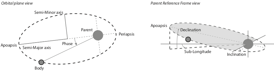
Parameters for orbiting body — **Fig. 2:** Sketch illustrating the orbital parameters of celestial bodies.

Radio Source Configuration

ON: Flag to activate the current radio source (true or false)
NAME: The name of the current radio source
PARENT: The name of the parent body for this source (must correspond to a defined BODY name)
TYPE: The type of radio source location. Four allowed values fixed in latitude, attached to a satellite, L-shell, M-shell.
LG_MIN: The lower bound value of the source longitude (in degrees)
LG_MAX: The upper bound value of the source longitude (in degrees)
LG_NBR: The number of steps for the source longitude.
LAG_MODEL: Model of the lead angle for the Io active flux tube; choices are: hess2011 [HBZG11], bonfond2009 [BGG+09], bonfond2017 [BGB+17], hinton2019 [HBB19], Hue2023 [HGL+23].
LAT: If Fixed in latitude: Latitude in degree; else: apex distance in planetary radii.
SUB: The subcorotation rate of the source (0 = no corotation)
AURORA_ALT: The altitude of the aurora (in planetary radii)
SAT: The name of the satellite when attached to a satellite is selected
NORTH: Flag to activate the Northern hemisphere source (exclusive with SOUTH item)
SOUTH: Flag to activate the Southern hemisphere source (exclusive with NORTH item)
WIDTH: The thickness of the radio emission sheet (in degrees)
CURRENT: The type of electron distribution in the source (see documentation). Allowed values: Transient (Alfvenic), Constant, Steady-State, Shell
CONSTANT: The value of beaming pattern half-cone opening angle (if Constant is selected), in degrees
MODE: The type of the wave mode. Allowed values: RX, LO (default is RX)
ACCEL: The value of resonant electron beam energy in keV (not used when Constant is selected)
TEMP: The value of the cold electron distribution temperature (in keV)
TEMPH: The value of the halo electron distribution temperature (in keV)
REFRACTION: Flag to activate refraction effects

Example: We configure a simulation with emission induced by Io ("TYPE": "attached to a satellite", "SAT": "Io"), in the northern ("NAME": "Source1", "NORTH": true) and the southern ("NAME"="Source2", "SOUTH": true) hemispheres. We use the lead angle model based on [hinton_JGR_20119] ("LAG_MODEL": "hinton2019") to determine the active magnetic field lines that will produce the emission. The electron have an energy of 3 keV ("ACCEL": 3) and the distribution function is of the loss cone type ("CURRENT": "Transient (Alfvenic)").

"SOURCE": [
  {

      "ON": true,
      "NAME": "Source1",
      "PARENT": "Jupiter",
      "TYPE": "attached to a satellite",
      "LG_MIN": 0,
      "LG_MAX": 0,
      "LG_NBR": 1,
      "LAT": 0,
      "LAG_MODEL":"hinton2019" ,
      "SUB": 0,
      "AURORA_ALT": 0.009091926738619804,
      "SAT": "Io",
      "NORTH": true,
      "SOUTH": false,
      "WIDTH": 1,
      "CURRENT": "Transient (Alfvenic)",
      "CONSTANT": 0.0,
      "MODE": "",
      "ACCEL": 3,
      "TEMP": 0,
      "TEMPH": 0,
      "REFRACTION": false
  },
  {
      "ON": true,
      "NAME": "Source2",
      "PARENT": "Jupiter",
      "TYPE": "attached to a satellite",
      "LG_MIN": 0,
      "LG_MAX": 0,
      "LG_NBR": 1,
      "LAG_MODEL":"hinton2019",
      "LAT": 0,
      "SUB": 0,
      "AURORA_ALT": 0.009091926738619804,
      "SAT": "Io",
      "NORTH": false,
      "SOUTH": true,
      "WIDTH": 1,
      "CURRENT": "Transient (Alfvenic)",
      "CONSTANT": 0.0,
      "MODE": "",
      "ACCEL": 3,
      "TEMP": 0,
      "TEMPH": 0,
      "REFRACTION": false
  }
]

Output Configuration

Dynamic Spectrum Output

Dynamic Spectra ouput setup:

INTENSITY: Flag to ouput ‘Intensity’ plots (true or false)
POLAR: Flag to ouput ‘Polar’ plots (true or false)
FREQ: Flags to setup output plot spectral axes
LONG: Flags to setup output plot longitude axes
LAT: Flags to setup output plot latitude axes
DRANGE: Distance range for plot setup (number, min and max)
LGRANGE: Longitude range for plot setup (number, min and max)
LARANGE: Latitude range for plot setup (number, min and max)
LTRANGE: Local-Time range for plot setup (number, min and max)
KHZ: Flag for spectral axis output in kHz (true or false, default is MHz)
LOG: Flag for spectral axis output in log scale (true or false)
PDF: Flag for PDF file output (true or false)
CDF: Configuration of CDF file output
- THETA: Flag for THETA parameter output in the CDF file (true or false)
- FP: Flag for FP parameter output in the CDF file (true or false)
- FC: Flag for FC parameter output in the CDF file (true or false)
- "AZIMUTH: Flag for AZIMUTH parameter output in the CDF file (true or false)
- OBSLATITUDE: Flag for OBSLATITUDE parameter output in the CDF file (true or false)
- SRCLONGITUDE: Flag for SRCLONGITUDE parameter output in the CDF file (true or false)
- SRCFREQMAX: Flag for SRCFREQMAX parameter output in the CDF file (true or false)
- OBSDISTANCE: Flag for OBSDISTANCE parameter output in the CDF file (true or false)
- OBSLOCALTIME: Flag for OBSLOCALTIME parameter output in the CDF file (true or false)
- CML: Flag for CML parameter output in the CDF file (true or false)
- SRCPOS: Flag for SRCPOS parameter output in the CDF file (true or false)
- SRCVIS: Flag for SRCVIS parameter output in the CDF file (true or false)
INFOS: IDL Saveset output (for debugging) (true or false)

2D Movie Output

ON: Flag to activate Movie2D generation (true or false)
SUBCYCLE: Subsampling rate of movie images (1=all temporal steps)
RANGE: Size of Field of view (in central body planetary radii)

3D Movie Output

ON Flag to activate Movie3D generation (true or false)
SUBCYCLE: Subsampling rate of movie images (1=all temporal steps)
XRANGE: Plotting Range in X axis (in central planet radius units)
YRANGE: Plotting Range in Y axis (in central planet radius units)
ZRANGE: Plotting Range in Z axis (in central planet radius units)
OBS: Flag to activate plotting the location of the observer
TRAJ: Flag to activate plotting the trajectories of the objects

Plasma Density Models

Various types of plasma density models can be used in ExPRES. They are configured by the DENS section in the BODY section (see the Celestial Body section above). Four types of density models are available:

Ionospheric: exponential decrease with distance,
Stellar: decreases with the distance squared,
Disk: exponential decrease with altitude relative to equatorial plane and radial distance,
Torus: exponential decrease from the center of a torus of given radius.

Plasma density model definitions include the following keywords:

ON: Set to true to activate the density model or to false deactivate.
NAME: The name of the density model (must be present, not empty and unique in the configuration file).
TYPE: The type of the density model, with the allowed values: Ionospheric, Stellar, Disk, Torus.
RHO0: Definition depends on density model type (see below).
SCALE: Definition depends on density model type (see below).
PERP: Definition depends on density model type (see below).

Ionospheric Model

The Ionospheric density profile is modeled as:

\[\rho = \rho_0 \exp\left(-\frac{r-(r_{ref}+h_0)}{H}\right)\]

where:

Parameter	Definition	Unit	Keyword
\(\rho_0\)	Reference plasma number density	\(\textrm{cm}^{-3}\)	`RHO0`
\(r\)	Radial distance	\(R_p\)
\(r_{ref}\)	Reference radial distance on ellipsoid	\(R_p\)
\(h_0\)	Peak density altitude above 1 bar level	\(R_p\)	`PERP`
\(H\)	Scale-height	\(R_p\)	`SCALE`

The \(r_{ref}\) is computed by ExPRES using the ellipsoid flattening parameter (FLAT keyword in BODY section) and the radio source latitude (computed from the SOURCE section).

Example: We define a Jovian ionospheric model, with a peak reference density of \(3.5\,10^5\,\textrm{cm}^{-3}\) at an altitude of 650 km above the 1 bar level (0.009092 \(R_p\)) and a scale height of 1600 km (0.0223801 \(R_p\)), as defined in [HTK98].

{
  "ON": true,
  "NAME": "Body1_density1",
  "TYPE": "Ionospheric",
  "RHO0": 350000.0,
  "SCALE": 0.0223801,
  "PERP": 0.009092
}

Stellar Model

The Stellar density profile is modeled as:

\[\rho = \rho_0 / r^2\]

where:

Parameter	Definition	Unit	Keyword
\(\rho_0\)	Reference plasma number density	\(\textrm{cm}^{-3}\)	`RHO0`
\(r\)	Radial distance	\(R_p\)

Note: Configuration keywords SCALE and PERP are not used for this model.

Disk Model

The Disk density profile is modeled as:

\[\rho = \rho_0 \exp\left(-\frac{r}{H_r}\right) \exp\left(-\frac{z}{H_z}\right)\]

where:

Parameter	Definition	Unit	Keyword
\(\rho_0\)	Reference plasma number density	\(\textrm{cm}^{-3}\)	`RHO0`
\(r\)	Equatorial radial distance	\(R_p\)
\(z\)	Altitude above equator	\(R_p\)
\(H_r\)	Equatorial radial scale-height	\(R_p\)	`PERP`
\(H_z\)	Vertical scale-height	\(R_p\)	`SCALE`

Torus Model

The Torus density profile is modeled as:

\[\rho = \rho_0 \exp\left(-\frac{\sqrt{(r-r_0)^2 + z^2}}{H}\right)\]

where:

Parameter	Definition	Unit	Keyword
\(\rho_0\)	Reference plasma number density	\(\textrm{cm}^{-3}\)	`RHO0`
\(r\)	Equatorial radial distance	\(R_p\)
\(z\)	Altitude above equator	\(R_p\)
\(r_0\)	Torus center equatorial diameter	\(R_p\)	`PERP`
\(H\)	Torus scale-height	\(R_p\)	`SCALE`

Example: We define the Io torus, with a peak reference density of \(2000\,\textrm{cm}^{-3}\), an equatorial diameter of 5.91 Jovian Radii (orbit of Io) and a torus scale-height of 1 Jovian radius, as defined in [Bag94].

{
  "ON": true,
  "NAME": "Body1_density2",
  "TYPE": "Torus",
  "RHO0": 2000,
  "SCALE": 1,
  "PERP": 5.91
}

Magnetic Field Models

The detailed magnetic field models available for ExPRES are listed in the LESIA_mag repository. We recall below the list of models and the related references.

Planet	Magnetic Field Model		Current Sheet Model		`BODY.MAG` Value
Planet	Short Name	Reference	Model Name	Reference	`BODY.MAG` Value
Mercury	A12	[AJK+12]			`A12`
Jupiter	JRM33	[CTO+22]	CON20	[CTHJ20]	`JRM33`
	ISaAC	[HBZG11]	CAN81	[CAN81]	`ISaAC+Connerney CS`
	JRM09	[CKO+18]			`JRM09+Connerney CS`
	O6	[Con92]			`O6+Connerney CS`
	VIP4	[CANS98]			`VIP4+Connerney CS`
	VIPAL	[HBBL17]			`VIPAL+Connerney CS`
	VIT4	[Con07]			`VIT4+Connerney CS`
Saturn	SPV	[DS90]			`SPV`
Saturn	Z3	[CAN84]			`Z3`
Uranus	AH5	[Her09]			`AH5`
Uranus	Q3	[CAN87]			`Q3`